

Time offsets#
This notebook introduces the concept of time offsets and how they are used in gwrefpy.
This notebook can be downloaded from the source code here.
Time offsets are a concept to handle time series with different timestamps. If two time series share the same timestamps, they can be compared directly. If not, we need to introduce a time offset to align them. The offset represents an interval for which all data points will be considered as having the same timestamp.
In the following notebook, we will illustrate this concept with a simple example. The example is inspired by section 3.3 in Strandanger (2024).
import gwrefpy as gr
import pandas as pd
import matplotlib.pyplot as plt
import warnings

gr.set_log_level("CRITICAL")
warnings.filterwarnings("ignore")
Log level set to CRITICAL
Data#
Let’s start by declaring the data we will explore as an example. We create Well objects and add to a Model object. Finally, we plot the data.
obs_ts = pd.Series(
    index=[
        pd.Timestamp("2023-01-07"),
        pd.Timestamp("2023-02-01"),
        pd.Timestamp("2023-02-25"),
    ],
    data=[10.4, 10.7, 10.8],
    name="obs",
)
ref_ts = pd.Series(
    index=[
        pd.Timestamp("2023-01-08"),
        pd.Timestamp("2023-02-03"),
        pd.Timestamp("2023-02-09"),
        pd.Timestamp("2023-02-25"),
        pd.Timestamp("2023-02-28"),
    ],
    data=[8.9, 9.2, 9.3, 9.3, 9.5],
    name="ref",
)
obs = gr.Well("obs", False, obs_ts)
ref = gr.Well("ref", True, ref_ts)

model = gr.Model("offset test")
model.add_well([obs, ref])

As we can see, the wells share some timestamps, but not all. In fact, only one timestamp (2023-02-25) is shared between the two wells. The table below shows an outer join between the two wells.
pd.concat([obs_ts, ref_ts], axis="columns", join="outer")
| obs | ref | |
|---|---|---|
| 2023-01-07 | 10.4 | NaN |
| 2023-01-08 | NaN | 8.9 |
| 2023-02-01 | 10.7 | NaN |
| 2023-02-03 | NaN | 9.2 |
| 2023-02-09 | NaN | 9.3 |
| 2023-02-25 | 10.8 | 9.3 |
| 2023-02-28 | NaN | 9.5 |
Using time offsets#
Our two wells have only one shared timestamp, but several timestamps that are close to each other. To compare the two time series, we can introduce a time offset.
A time offset defines a ±offset window around each observation time point. All reference points falling within that window are aggregated (mean by default) into a single matched value for that observation. This is called the anchor method, and it is the default since version 1.0.0.
Important
The offset extends in both directions. For example, given an observation timestamp of 2023-02-25 and an offset of 3 days, all reference points between 2023-02-22 and 2023-02-28 will be matched to that observation.
The offset argument can be given as a string or a pandas.Timedelta object. Refer to the pandas documentation for more information about accepted strings.
As of version 0.2.0 the aggregation within an offset can be set to "mean" (default), "median", "min", or "max" (see the API reference for the Model class and its fit method).
Grouping methods#
Two grouping methods are available via the method parameter:
"anchor"(default): each observation time is the center of a±offsetwindow; all reference points inside that window are aggregated into one output pair per observation. Works reliably for both sparse and dense/high-frequency reference data."consecutive": all timestamps from both series are merged, sorted, and split into groups wherever the gap between consecutive timestamps exceedsoffset. Both reference and observation values within each group are aggregated. This was the default prior to version 1.0.0, and remains available for very sparse, irregular monitoring data where the chaining behaviour is intentional.
Analysing offsets#
We provide a helper function for analysing multiple time offsets at once: analyze_offsets. This function takes a list of offsets and returns the number of matching data pairs. analyze_offsets(obs, ref, ...) uses the obs timestamps as anchors, so it answers the question: “for how many observation measurements can a matching reference be found?” Both methods are supported via the method parameter (default "anchor").
Let’s analyse offsets of 0, 1, and 3 days.
offsets = ["0D", "1D", "3D"]
results = gr.analyze_offsets(obs, ref, offsets)
results
| n_pairs | |
|---|---|
| offset | |
| 0D | 1 |
| 1D | 2 |
| 3D | 3 |
Let’s plot the width of the offset to understand the results better.

For this simple example, a time offset of 3 days seems reasonable.
With the default anchor method and offset="3D", each observation timestamp is the center of a ±3D window:
Period 1 (January): obs
2023-01-07window spans Jan 4–10. Ref2023-01-08is 1 day away → one matched pair.Period 2 (early February): obs
2023-02-01window spans Jan 29–Feb 4. Ref2023-02-03is 2 days away → matched. Ref2023-02-09is 8 days away → not matched. One matched pair.Period 3 (late February): obs
2023-02-25window spans Feb 22–28. Both ref2023-02-25(0 days) and ref2023-02-28(3 days) fall inside → both are aggregated into one pair (mean of 9.3 and 9.5 = 9.4).
Fitting produces 3 data pairs — one per observation point.

When fitting these two wells with an offset of 3 days, three data pairs will formed as explained above.
Shifting timeseries#
It is possible to shift the timeries of an observation well to accout for delays in the response.
We will import the deviations exampel and shift the obervation well with 10 days.
model = gr.Model("small_example.gwref")
model.well_names
model.fits = []

obs_well = model.obs_wells[0]
ref_well = model.ref_wells[0]
# shift the time for this example
shift = pd.Timedelta("-10D")
obs_well.timeseries = obs_well.shift_timeseries(shift)

model.plot_wells()
(<Figure size 1000x600 with 1 Axes>,
 <Axes: title={'center': 'Wells Plot'}, xlabel='Time', ylabel='Measurement'>)
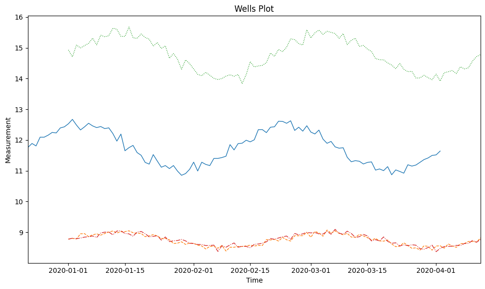
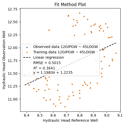
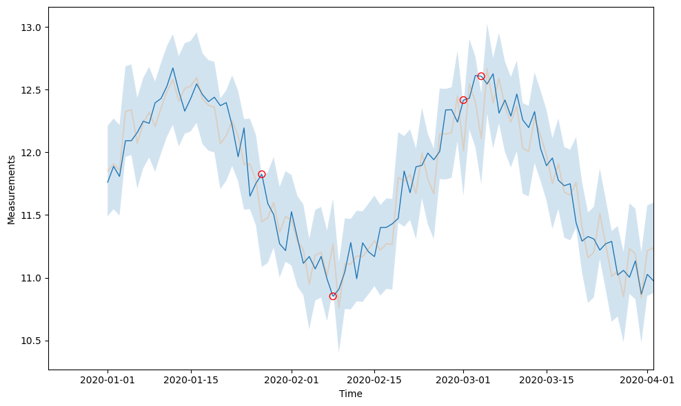
The fit of the two wells are now
fit0 = model.fit(obs_well=obs_well, ref_well=ref_well, offset="0D")
model.plot_fitmethod(fit0)
model.plot_fits(fit0)
(<Figure size 1000x600 with 1 Axes>,
 <Axes: xlabel='Time', ylabel='Measurements'>)
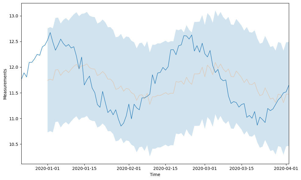
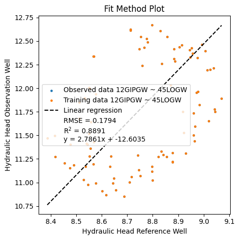
and we can compare this fit with another one with a shift
fit1 = model.fit(obs_well=obs_well, ref_well=ref_well, offset="0D", shift="10D")
model.plot_fitmethod(fit1)
model.plot_fits(fit1)
(<Figure size 1000x600 with 1 Axes>,
 <Axes: xlabel='Time', ylabel='Measurements'>)
This concludes this notebook on time offsets in gwrefpy. Happy fitting!